Time Response of Second Order Transfer Function and Stability Analysis

Time Response of Second Order Transfer Function and Stability Analysis

In this article we will explain you stability analysis of second-order control system and various terms related to time response such as damping (ζ), Settling time (t_s), Rise time (t_r), Percentage maximum peak overshoot (% M_p), Peak time (t_p), Natural frequency of oscillations (ω_n), Damped frequency of oscillations (ω_d) etc.

1) Consider a second-order transfer function = . (Do you know why it is second order transfer function; the reason is, the highest power of ‘s’ in the denominator is two). We will call it system-1 in the subsequent discussion.

The standard form of a second-order transfer function is given by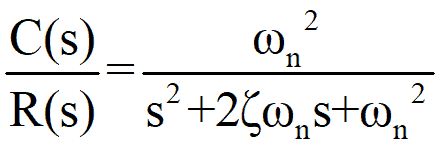

If you will compare the system-1 with standard form, you can find that damping ‘ζ’= 0.2 (damping is a unitless quantity), Natural frequency of oscillations ‘ω_n’= 4 rad/sec.

Various time domain specifications their definitions, formula and calculations for the given system are as follows:

Delay time (t_d):

It is the time required for the response to reach half of its final value from the zero instant. It is denoted by t_d.

t_d= = 0.285 seconds.

Rise time (t_r):

Rise time refers to the time required for a signal to change from a specified low value to a specified high value. In case of underdamped system time required for the response to rise from 0% to 100% is called rise time. It is denoted by t_r.

t_r= = 0.452 seconds.

Settling time (t_s):

It is the time required for the response to reach the steady state and stay within the specified tolerance bands around the final value. In general, tolerance bands are 2% and 5%. The settling time is denoted by t_s. In this article formula and calculation of settling time is based on 2% tolerance band.

t_s = = 5 seconds.

Percentage maximum peak overshoot (% M_p):

It is the percentage difference in the first peak of time response and steady-state output value.

 % M_p = = 52.66%

Peak time (t_p):

The peak time is the time required for the response to reach the first peak of the overshoot. The settling time is denoted by t_p.

t_p= = 0.802 seconds

Damped frequency of oscillations (ω_d):

ω_d= = 3.919 rad/sec. It is equal to the imaginary part of the poles of the transfer function.

Poles of the transfer function (roots of the denominator):

-0.8±j3.92; also called roots of characteristics equation.

In figure-1, few of the above-calculated values are shown in a complex plane (s-plane), so you can understand, what the relation between them are.

Time response of system-1, against unit step input, is as shown in figure-2,

From figure -2 and definitions of Time response specifications such as delay time, rise time, peak time, etc. you can understand their significance. Theoretical values calculated are shown in figure-2. The first peak can be viewed between 1.4 and 1.6. The exact point is 1.5266 (not shown in the figure), hence the %M_p is 52.66%. If you will calculate the time period of one cycle, reciprocate it, it will be frequency in Hertz, multiply it by 2π, now it is in rad/sec.; you will find it is equal to ω_d. (If you will generate this graph from software’s, then you can zoom the graph and verify all the values such as  %M_p, ω_d, t_p, t_r, t_d, etc.).

To understand the term settling time ‘t_s’, refer figure 3.

Time response shown in figure-2 is just reproduced in figure-3, but with a change in the y-axis. In figure-3, y-axis is from 0.98 to 1.02 (2% range of final value).

Perhaps you may think that the time required until all the oscillations are completely damped out (vanished) is called settling time; no, it is not true. Oscillations may be continued after settling time. In the case of step input, the time required to decrease the oscillations within two percent range of input is called settling time. In the present case, the steady-state value of the input is ‘1’.

From figure-3, it can be viewed that after 5 seconds oscillations are within two percent range of input value, hence settling time is five seconds. Same is calculated theoretically.

So, with the above discussions, you might have understood about various time domain specifications.

Now, please note the following points regarding stability:

1. Stable systems have positive damping, marginally stable systems have zero damping and unstable systems have negative damping. In the present example damping is 0.2, hence the system is stable.
2. If the damping is between zero to one then poles of the closed-loop transfer function will be complex. It is called underdamped system. System-1 is the example of an underdamped system.
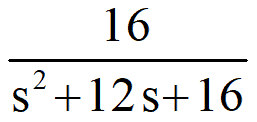
3. If the damping is one, then it is called critically damped system. For example transfer function =    is an example of a critically damped system. You can find it has ‘ζ’= 1, ‘ω_n’= 4 rad/sec. The system has two real roots both at ‘-4’.
4. If the damping is more than one, then it is called overdamped system (i.e. damping is in excess). Critically damped and overdamped systems don’t have oscillations.

Transfer function  =  is an example of an overdamped system. You can find it has ‘ζ’= 1.5, ‘ω_n’= 4 rad/sec. The system has two real roots both are real and unequal.

• A good control system should have damping around 0.7-0.9. (In fact, if the damping is one, then it is the best system, but it is very difficult to achieve accurate damping. Suppose a system has damping 0.2, then with the help of PD Controllers, Lead compensation, etc., damping can be increased. Designing of controllers is also a vast research topic. Designing should be such that damping should be increased to 0.7-0.9 from 0.2. If the damping is increased to 0.99 or 1, then it will be better. But as written earlier accurate damping cannot be achieved and if it is more than one, then it will be overdamped. Hence it is better to maintain the damping around   7-0.9.
• If you will draw time response of a critically damped and overdamped system and compare it, you will find that overdamped system has higher settling time; hence over damping is not acceptable. Exact damping ‘1’ cannot be maintained, therefore damping should be slightly below ‘1’. In other words, we can say, Poles of the closed loop transfer function (Roots of characteristics equation) should be complex and have a slight (little) imaginary part. In the time response of the system, there should be slight oscillations. Value of ω_d should be low but not zero.
• If poles are away from imaginary axis in LHS, then the system is more stable, i.e. the value of ζ ω_n should be high (refer figure-1); or we can say high value of ζ ω_n will result in low settling time, low transient period, hence better stability.

Now we will compare various second order transfer function to further explain the stability.

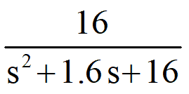
2) Consider another transfer function (system-2): =    

Its poles (i.e. roots of the denominator) are: -1.25 ±j3.80.   ζ= 0.3125, ω_n= 4 rad/sec

Against unit step input its time response is:

Now try to compare both the systems: system-1 and system-2. Which system is more stable & why?

The answer is system-2 have better stability. The reasons are:

• Poles of the closed loop transfer function are away from the imaginary axis as compared to system-1 (i.e. system-2 has more negative real part).
• Damping is higher than system-1.
• From time response it can be viewed, system-2 has less peak overshoot and settling time (transient period) as compared to system -1.

3) Now consider another transfer function (system-3):  =   .

Its poles are: 0±j4; damping ‘ζ’= 0, Natural frequency of oscillations ‘ω_n’= 4 rad/sec.

Its time response against unit step input is:

It is a marginally stable system; also called the undamped system. Do you know, why? The reasons are:

• Poles are at the imaginary axis (real part is zero)
• From time response, it can be seen that oscillations are neither decaying nor growing. (It is also called sustained oscillations)
• Damping is zero
• In the transfer function, one coefficient is missing (s¹ is missing)
• If Routh Hurwitz criterion is applied in the denominator of a transfer function, it can be found that one row is zero.

4) Now consider one more transfer function (system-4): =   .

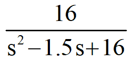Its time response against unit step input is shown in figure-6 as below:

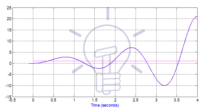
It is an unstable system, because of the following reasons:

• If poles are calculated, then it can be found that poles are at Right-hand side (RHS) of the imaginary axis (real part of the poles is positive).
• From time response, it can be seen that oscillations are growing.
• Damping is negative.
• In the denominator of the transfer function, there is a sign change.
• Also, From the Routh Hurwitz criterion, it can be found that the system is unstable.

5) Now consider another transfer function = 

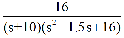
It is also an unstable system, because of the following reasons. The poles of this system are -10, 0.75±j3.93. Though one pole is at LHS of s-plane but for the stability of the system, all the poles must be at LHS, not a single pole can be at RHS of s-plane.

To compare the stability of all the systems mentioned above, there is one more method; it is the calculation of Gain margin (GM) & Phase margin (PM). Now we will discuss this method.

System-1 can be represented as follows:

(It is assumed that it is a unity feedback system)

Its open loop transfer function (also called open loop gain) is G(s)H(s)=

Its GM & PM can be found from bode plot, polar plot or directly from software such as MATLAB.

GM & PM of system-1 is found to be: GM= ∞ db PM= 22.6°.

Similarly for the system-2, open loop transfer function: G(s)H(s)=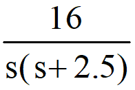

Its GM=∞ db & PM= 34.6 °.

In both, the above cases GM cannot be compared (as both the systems have GM infinity), but It can be observed that PM is higher in case of system-2; it is another reason that system-2 has better stability.

For the system-3, open loop transfer function: G(s)H(s)=

It’s GM= PM= 0; it is another reason that system-3 is marginally stable.

For the system-4, open loop transfer function G(s)H(s)=

One pole of its open loop transfer function is at RHS, in such cases calculation of GM, PM is not a suitable method to find the stability.

Now, please note the following statement:

Gain margin (GM) & Phase margin (PM) are positive if the system is stable, negative if the system is unstable and both are zero if the system is marginally stable. Higher the GM & PM, more the system is stable (This is the reason, measurement of GM & PM is called relative stability).

[Above statement is true if not a single pole of the open loop transfer function is in RHS of s-plane.  Let, in a system In such type of systems, above statement of GM & PM is not true. In this case, open loop transfer function has one pole at RHS of s-plane, but the system is stable. You can write its characteristics equation and verify it through Routh Hurwitz Criterion. Explanation of Such type of systems is given in the Nyquist Stability Criterion].

So, with the above definition of GM & PM, you can compare the stability of systems 1-3.

Analysis of GM & PM is called frequency response method. In control engineering books, you will find that time response and frequency response are separate chapters; but for better understanding of stability and comparison of different systems, GM & PM are included in this article.

About the Author

Dr. Vipin Jain obtained degree of Bachelor of Engineering in 1992 from Nagpur University, Master of Technology in 2007, Ph.D. Degree in 2017 from University of Delhi. He has long teaching and industrial experience. He is a faculty member in the Electrical Engineering Department, Bharat Institute of Technology, Meerut (UP), India, since December 2007. More than twenty research papers have been published by him so far. He is energy auditor certified by Bureau of Energy Efficiency, Government of India.

Related Posts:

• Quantization & Sampling? Types & Laws of Compression
• What is Negative Feedback?
• Design & Installation of Control & Monitoring Systems in Electrical Engineering