Nyquist Stability Criterion – Examples and MATLAB Coding
Nyquist Stability Criterion – MATLAB Code with Examples
The Nyquist criterion is widely used in electronics and control system engineering, as well as other fields, for designing and analyzing systems with feedback. While Nyquist is one of the most general stability tests, it is still restricted to linear, time-invariant (LTI) systems.
The most common use of Nyquist plots is for assessing the stability of a system with feedback. In Cartesian coordinates, the real part of the transfer function is plotted on the X-axis. The imaginary part is plotted on the Y-axis. The frequency is swept as a parameter, resulting in a plot per frequency.
Nyquist Stability Criterion can be expressed as
Z = N+P
Where: Z= number of roots of 1+G(s)H(s) in the right-hand side (RHS) of s-plane (It is also called zeros of characteristics equation)
N=number of encirclement of critical point 1+j0 in a clockwise direction
P=number of poles of open loop transfer function (OLTF) [i.e. G(s)H(s)] in RHS of s-plane.
Above condition (i.e. Z=N+P) is valid for all systems whether stable or unstable.
Now we will explain this criterion with the following examples:
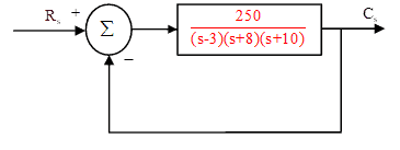
Example 1:
Consider an open loop transfer function (OLTF) as:![]() We will call it system-1 in the subsequent discussion. It is a stable system or unstable? Perhaps few of you will say that it is an unstable system because one pole is at +3, but it should be noted that stability depends on the denominator of a closed-loop transfer function;
We will call it system-1 in the subsequent discussion. It is a stable system or unstable? Perhaps few of you will say that it is an unstable system because one pole is at +3, but it should be noted that stability depends on the denominator of a closed-loop transfer function;![]() If any one of the roots of the denominator of a closed-loop transfer function (also called roots of characteristics equation; or say poles of closed-loop transfer function) is at RHS of s-plane then the system is unstable. So in above case pole at +3 will try to bring the system towards instability, but it is not necessary that the system is unstable. First, we will analyze that this system is stable or not, then we will discuss the Nyquist Stability Criterion.
If any one of the roots of the denominator of a closed-loop transfer function (also called roots of characteristics equation; or say poles of closed-loop transfer function) is at RHS of s-plane then the system is unstable. So in above case pole at +3 will try to bring the system towards instability, but it is not necessary that the system is unstable. First, we will analyze that this system is stable or not, then we will discuss the Nyquist Stability Criterion.
- The complete control system mentioned in this example is shown in Figure-1 [assuming that it is a unity feedback control system; i.e. H(s)=1].
Against unit step input its time response is shown in Figure-2.

From Figure-2, it can be easily understood that the system is stable.
- Characteristics equation of a control system is given as:
1+G(s)H(s)=0,
So, in this system characteristics equation is 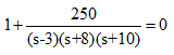
or,
s3+ 15s2+ 26s+10 = 0
Its roots are: -13.0691, -1.3740, -0.5569; as all the roots are in left-hand side (LHS) of s-plane hence the system is stable.
- From Routh Hurwitz criterion also, its stability can be verified.
From Figure-2, it can be seen that the system has no oscillations. The reason is, it is an overdamped system. Pole at ‘-13.0691’ can be ignored (poles far away from the imaginary axis have less influence while poles near to the imaginary axis have more influence; hence poles near to the imaginary axis are also called dominant poles); so remaining system is second order control system and now two remaining roots are different and have no imaginary part hence system is overdamped. To understand overdamped system refer article Time Response of Second-order Transfer Function and Stability analysis (or, you can understand it like this also, ignore two poles -13.0691, -1.3740, consider only one pole -0.5569, as it is the dominant pole. Now it is the first order control system or say first order transfer function. Time response shown in Figure-2 is very similar to the response of first-order transfer function against step input.)
In the article Time Response of Second order Transfer Function and Stability analysis, it is shown that Gain margin (GM) & Phase margin (PM) indicates about the stability of the system.
If Gain margin (GM) & Phase margin (PM) is positive then the system is stable, if negative than the system is unstable and if both are zero then the system is marginally stable. Higher the GM & PM, more the system is stable.
But note that the above statement is true if not a single pole of the open loop transfer function is in RHS of s-plane. In the system-1 one pole is at ‘+3’, i.e. one pole of the open loop transfer function is at RHS of s-plane; in such type of systems Nyquist plot and Nyquist Stability Criterion is a very useful tool for the analysis of a system.
Nyquist plot of system-1 is as follows:

From the OLTF, you can understand, P=1, (one pole of the OLTF is at RHS of s-plane)
N=-1, N is the number of encirclement of critical point 1+j0 in a clockwise direction, in Figure-3, a critical point is encircled once in an anti-clockwise direction.
As Z=N+P, hence Z=0;
i.e. number of roots of characteristics equation in RHS of s-plane is zero, therefore, the system is stable.
(if the value of Z is other than zero then the system will be unstable. Z cannot be negative).
Example 2:
Now take another example: ![]()
We will call it system-2.
The Nyquist plot of system-2 is as shown in Figure-4.

So, from the Nyquist plot, it can be viewed that N=0. (No encirclement of critical point by Nyquist plot)
In this example also P=1. (one pole of OLTF is at RHS; i.e. one pole is at +3)
So, Z=N+P=1; therefore one pole of a closed-loop transfer function is at RHS of s-plane, hence the system is unstable.
(You can find roots of characteristics equation. It will be -11.7862, -5.4096, 2.1958; you can understand because of 2.1958, the system is unstable).
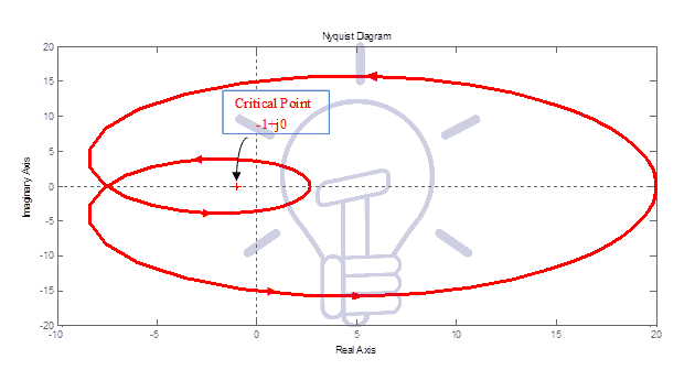
Example 3:
Now take another example: 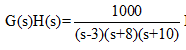 Here again P=1.
The nyquist plot is as follows (Figure-5):

You can see N=1. (Encirclement of the critical point is once in a clockwise direction).
Z=N+P=2, therefore two roots of characteristics equation is in RHS of complex plane (s-plane)
(Roots of characteristics equation are -16.2724, 0.6362 ±j 6.8044; i.e. Z=2; two poles 0.6362 ±j 6.8044 are at RHS of s-plane).
So, you can understand, condition Z=N+P is valid for all the systems.
Example 4:
Now Consider 
If you will draw its Nyquist plot, it will pass through a critical point (–1+j0). In this case, the system is marginally stable. You can understand ‘N’ is undefined in this case (In the present case two roots of characteristics equation will be at origin and one root on Left Hand Side of s-plane. Therefore the system will be marginally stable).
Summary of Systems 1-4:
In all the above examples you can see that denominator is same, but the numerator is different, or say numerator is variable. So, Keep ‘K’ in the numerator instead of a fixed value; hence consider the following open loop transfer function:

If you will apply the Routh Hurwitz criterion to characteristics equation 1+G(s)H(s), then you will find the range of ‘K’ as 240<K<630
So, now you can understand why systems in examples 1–4 are stable, unstable or marginally stable.
You can draw the root locus of the above transfer function, it will be as shown in Figure-6

(It can be seen that branches of Root locus plot are starting from 3, -8, -10, where K=0. So you can see for K<240, two poles of closed-loop transfer function will be at LHS of s-plane, but one pole will be at RHS of s-plane, hence for K<240 system is unstable.
As the system is stable for 240<K<630, so, If you will decide K=250, then it will be system-1 (example-1), in this case, all the poles of the closed loop transfer function are real and in the LHS of s-plane and the system is stable. If you will decide K=1000, then it will be system-3 (example-3), then two poles of the closed loop transfer function are complex and one pole is real; but the system will be unstable. For Further understanding you can refer Root Locus articles)
It is the Nyquist criterion article, but root locus plot is inserted for better understanding. In examples 1-4, the only difference in open loop transfer function is that numerator is variable, so we have written ‘K’ instead of a fixed value and root locus is drawn. You can understand by the movement of ‘K’, what will be the effect on poles of a closed-loop transfer function.
Now we will take up a few more examples:
Example 5:
Consider 
Its Nyquist Plot is as follows:

As per the transfer function P=0 (no pole of OLTF on RHS)
As per the Nyquist plot N=0 (No encirclement of critical point by Nyquist plot).
Hence Z=N+P=0; implies that no pole of a closed-loop transfer function is in RHS of s-plane, hence the system is stable.
Example 6:
Consider 
Its Nyquist Plot is as follows:
As per the transfer function P=2 (two poles of OLTF on RHS)
As per the Nyquist plot N=–2
Hence Z=N+P=0; implies that no poles of the closed-loop transfer function in RHS of s-plane, hence the system is stable.
- Please note that in this article, formula Z=N+P is used, where N=number of encirclement of critical point 1+j0 in a clockwise direction. In a few books, you may find the formula Z=–N+P, where N=number of encirclement of critical point 1+j0 in a counter-clockwise direction. Both are correct.
MATLAB Coding:
We are writing here MATLAB coding also, so that readers can generate Nyquist Plot and verify all the results.
MATLAB coding to generate a Nyquist plot is as follows:
s=tf(‘s’)
G1=250/ ((s-3)(s+8)(s+10))
nyquist(G1)
% above command will generate Nyquist plot of example-1
% G1 is a variable, you can type sys1, system1, etc. instead of G1
G2=100/ ((s-3)(s+8)(s+10))
nyquist(G2)
% above command will generate Nyquist plot of example -2
Similarly, Nyquist plots of all the systems can be generated.
Through the command: s=tf(‘s’), letter ‘s’ is treated as operator ‘s’ of Laplace function. No need to give this command every time. Once you will shut down the MATLAB and reopens it, then only you have to execute this command.
Related Posts: