Norton’s Theorem in DC Circuit Analysis
Norton’s Theorem is another useful technique for analyzing electric circuits, similar to Thevenin’s Theorem. Both methods simplify linear, active circuits and complex networks into an equivalent circuit. The main difference between Thevenin’s and Norton’s theorem is that Thevenin’s Theorem represents the circuit as an equivalent voltage source in series with an equivalent resistance. On the other hand, Norton’s Theorem represents it as an equivalent current source in parallel with an equivalent resistance.
Norton’s Theorem states that:
Any linear electric network or complex circuit with current and voltage sources can be replaced by an equivalent circuit containing a single independent current source IN and a parallel resistance RN.
In simple terms, any linear circuit can be represented as a real, independent current source connected to a specific pair of terminals.
Good to Know:
Norton’s theorem was independently derived in 1926 by Hans Ferdinand Mayer and Edward Lawry Norton. Mayer, a German researcher at Siemens and Halske, and Norton, an American engineer at Bell Labs, arrived at the same conclusion around the same time.
Related Post: Thevenin’s Theorem. Easy Step by Step Procedure with Example (Pictorial Views)
Steps to Analyze an Electric Circuit using Norton’s Theorem
- Short the load resistor.
- Calculate / measure the short circuit current. This is the Norton Current (IN).
- Open all current sources, short all voltage Sources and open the load resistor.
- Calculate /measure the open circuit resistance. This is the Norton Resistance (RN).
- Redraw the circuit with the measured short-circuit current (IN) from Step (2) as the current source and the measured open-circuit resistance (RN) from Step (4) as the parallel resistance. Then, reconnect the load resistor that was removed in Step (3). This forms the Equivalent Norton’s Circuit of the linear electrical network or complex circuit to be simplified and analyzed. You’re done!
- Find the load current (IL) flowing through the load resistor and the load voltage (VL) across it by applying the current divider rule:
(IL = IN / (RN / (RN+ RL)
The load voltage can then be calculated as:
VL = IL × RL
For a clear explanation, refer to the solved example given below.
Solved Example by Norton’s Theorem:
Example:
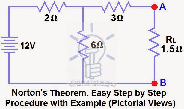
Using Norton’s Theorem, determine RN, IN, the current flowing through the load resistor, and the load voltage across it in Figure (1).
Solution:-
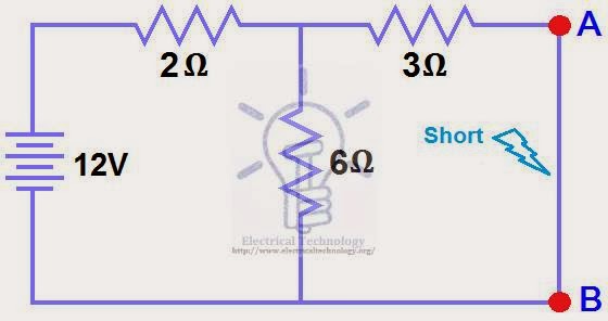
STEP 1.
Short the 1.5Ω load resistor as shown in (Fig 2).
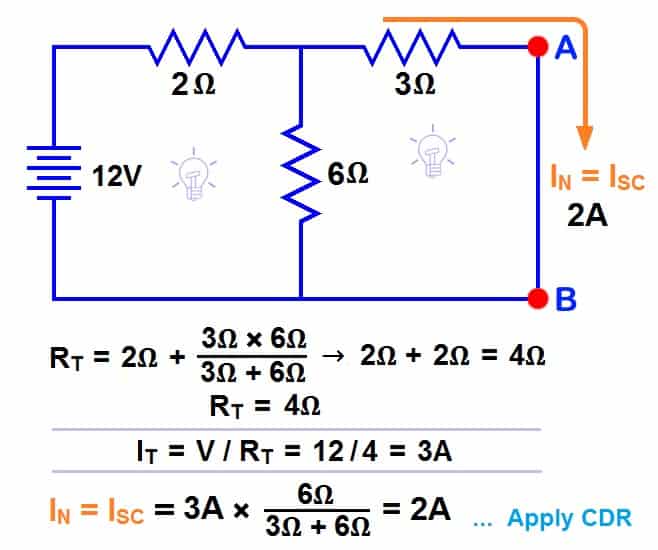
STEP 2.
Calculate / measure the Short Circuit Current. This is the Norton Current (IN).
To determine the Norton current (IN), we short the AB terminals. The 6Ω and 3Ω resistors are now in parallel, and this parallel combination is in series with the 2Ω resistor.
So, the total resistance of the circuit to the source is:-
2Ω + (6Ω || 3Ω) ….. (|| = in parallel with).
RT = 2Ω + [(3Ω x 6Ω) / (3Ω + 6Ω)] → IT = 2Ω + 2Ω = 4Ω.
RT = 4Ω
IT = V ÷ RT
IT = 12V ÷ 4Ω
IT = 3A.
Now we have to find ISC = IN … Apply CDR… (Current Divider Rule)…
ISC = IN = 3A × [(6Ω ÷ (3Ω + 6Ω)] = 2A.
ISC = IN = 2A.
STEP 3.
Open the current source, short the voltage source, and remove (open) the load resistor, as shown in Figure (4).
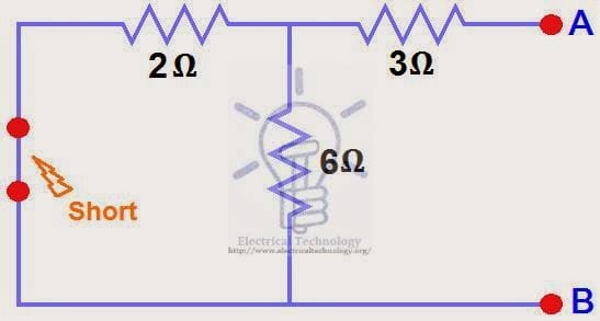
STEP 4.
Calculate /measure the open circuit resistance. This is the Norton Resistance (RN)
In Step (3), we reduced the 12 V DC source to zero, which is equivalent to replacing it with a short circuit, as shown in Figure (4). We can see that the 3Ω resistor is in series with the parallel combination of the 6Ω and 2Ω resistors, i.e.:
3Ω + (6Ω || 2Ω) ….. (|| = in parallel with)
RN = 3Ω + [(6Ω × 2Ω) ÷ (6Ω + 2Ω)]
RN = 3Ω + 1.5Ω
RN = 4.5Ω

STEP 5.
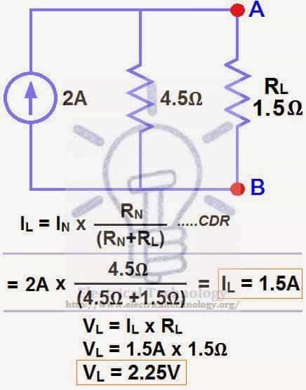
Connect RN in parallel with the current source IN, and then reconnect the load resistor, as shown in Figure (6). This represents the Norton Equivalent Circuit with the load resistor connected.

STEP 6.
Finally, apply the last step i.e. calculate the load current through, and the load voltage across, the load resistor using Ohm’s Law, as shown in Figure (7).
Load Current through Load Resistor…
IL = IN x [RN ÷ (RN+ RL)]
= 2A × (4.5Ω ÷ 4.5Ω + 1.5Ω) → = 1.5A
IL = 1. 5A
And
Load voltage across the load Resistor…
VL = IL × RL
VL = 1.5A × 1.5Ω
VL= 2.25V
Now compare this simplified circuit with the original circuit in Figure (1). Can you see how much easier it becomes to measure or calculate the load current and load voltage for different load resistors using Norton’s Theorem, even in much more complex circuits? The answer is: only and only yes.
Good to Know: Both Norton’s and Thevenin’s Theorems can be applied to both AC and DC circuits containing different components such as resistors, inductors, and capacitors. In AC circuits, the Norton current (IN) is expressed as a complex number (polar form), whereas the Norton resistance (RN) is stated in rectangular form.
- Related Posts:
- Maximum Power Transfer Theorem for AC & DC Circuits
- Kirchhoff’s Current & Voltage Law (KCL & KVL) | Solved Example
- Compensation Theorem – Proof, Explanation and Solved Examples
- Substitution Theorem – Step by Step Guide with Solved Example
- Millman’s Theorem – Analyzing AC & DC Circuits – Examples
- Superposition Theorem – Circuit Analysis with Solved Example
- Tellegen’s Theorem – Solved Examples & MATLAB Simulation
- SUPERNODE Circuit Analysis | Step by Step with Solved Example
- SUPERMESH Circuit Analysis | Step by Step with Solved Example
- Voltage Divider Rule (VDR) – Solved Examples for R, L and C Circuits
- Current Divider Rule (CDR) – Solved Examples for AC and DC Circuits
- Star to Delta & Delta to Star Conversion. Y-Δ Transformation
-
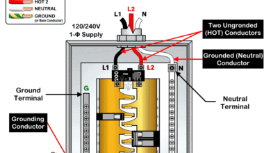 Difference Between Grounding, Grounded and Ungrounded Conductors
-
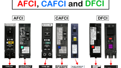 Difference Between AFCI, CAFCI, DFCI and GFCI?
-
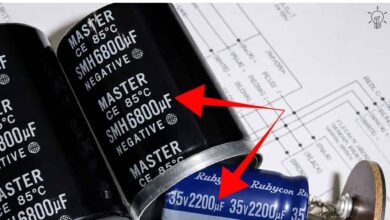
 Why is a Capacitor Bank Rated in kVAR, Not in Farad?
-
 Why is the Rating of a Capacitor Expressed in Farad?
-
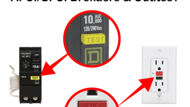 What Happens When You Press TEST and RESET on a GFCI
-
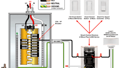 Wiring Z-Wave Smart Switch, Dimmer & Fan Speed Controller