An introduction to Maximum Power Point Algorithms in PV Systems
Maximum Power Point (MPPT) Algorithms – Fractional Open Circuit Voltage & Perturb and Observe Methods
In a solar photovoltaic system, every PV module has an operating point which is decided by the load to which it is connected. This operating point varies throughout the day as the irradiance falling on the module varies. It is desired to transfer the maximum available power from the PV array to the load at the available irradiance. To understand this let’s take a look at figure 1 shown below.
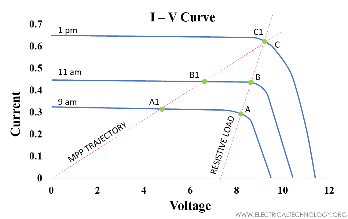
Points A1, B1, and C1 represent the points at which the module will provide maximum power at 9 am, 11 am, and 1 pm respectively. Whereas points A, B, and C represents the actual operation of the PV modules at different irradiance available at 9 am, 11 am, and 1 pm respectively.
Related Post:
- What is a Solar Charge Controller? Selecting the Right Size of MPPT & PWM Charge Controllers
- Basic Components Needed for Solar Panel System Installation
The PV power output available at A1, B1, and C1 is less than the output at A, B, and C respectively. So instead of operating at maximum power the operating point of the PV module is far below its maximum power point. Thus, to extract the maximum power at the available irradiance from the PV array a special method called Maximum power point Tracking (MPPT) is adopted.
Unlike mechanical tracking, the maximum power point tracking includes a power electronic circuit which ensures that the PV module operates at the maximum power point. This method of tracking involves an electronic circuit and an algorithm that work on the idea of impedance matching.
The condition of impedance matching between the load and the PV source is necessary to operate the module at maximum power. This is commonly done by using a DC-DC converter, in this the power from the solar module is calculated which is an input to the MPPT algorithm (or Maximum Power Point Algorithms) and the duty cycle adjustment of the semiconductor switch in the converter is the output of that algorithm.
By adjusting the duty cycle of the semiconductor switch we are controlling the average current flow which will force our PV module to operate at the desired operating power which corresponds to the maximum power of the PV module during the available irradiance. Now let us take a look at some of the MPPT (Maximum Power Point) algorithms.
- Fractional Open Circuit Voltage method
- Perturb and Observe method
Related Posts:
Fractional Open Circuit Voltage Method:
The fractional open circuit voltage method takes an advantage of the fact that the ratio of module voltage at maximum power point (VMP) to module voltage at open circuit (VOC) is constant i.e., VMP/ VOC = 0.78. This constant is also referred to as K and it differs from cell technology used. In standard PV modules the VMP is around 78% of the VOC.
In this method, the PV array voltage is sensed and then this sensed value of voltage is compared with the reference value of voltage. i.e., VMP = 0.78 × VOC this generates an error signal which is utilized to generate pulses of the control signal by comparing it with a triangular wave which adjusts the duty cycle of the converter to achieve the maximum power point at VMP.
Since there is a change in the irradiance the module VOC changes with the change in irradiance therefore method requires measuring the VOC during the operation. This can be done by temporarily disconnecting the PV module during operation. However, this would result in the loss of power. This could become worse if the irradiance changes rapidly.
Another way is to measure VOC by connecting a cell in parallel to the PV modules (which would have the same temperature and irradiance as that of the module). This is also referred to as a pilot cell. This cell voltage is used as VOC which is further used to track the maximum power point on the PV curve. This method is simple as compared to the other complicated technique. But the constant K is just an approximation that does not point us to the true maximum power point but gets us close in the region of the maximum power point.
Related Posts:
- How Much Watts Solar Panel You Need for Home Appliances?
- A Complete Guide About Solar Panel Installation. Step by Step Procedure with Calculation & Diagrams
Perturb and Observe Method
Perturb and observe method, falls in the category known as hill climbing maximum power point algorithm. In this algorithm, perturbation is provided to the array/module voltage by increasing or decreasing the duty cycle of the switching semiconductor device. This change in the duty cycle would cause the voltage to increase or decrease. Take a look at the PV curve shown in figure 2 below.

If the increase in the voltage results in the increase of the module input power (compared to the old power of PV module) as shown in the PV curve arrow A, then the present operating point lies to the left of the maximum power point and hence further perturbation of voltage is needed towards the right to reach maximum power point by further varying the duty cycle of the switching device.
Whereas on the contrary if an increase in the voltage causes the module input power to decrease as shown in the PV curve arrow B, then the present operating point is towards the right of the maximum power point, and a reduction in the voltage has to be done by varying the duty cycle of the switching device to reach the maximum power point.
Similarly, if a decrease in voltage results in the increase of the module input power as shown in the PV curve arrow C, then the present operating point lies to the right of the maximum power point, and hence further perturbation of voltage is needed towards the left to reach maximum power point by varying the duty cycle.
If a decrease in voltage causes the input power to decrease as shown in the PV curve arrow D, then our operating point lies to the left of the maximum power point and hence perturbation of voltage has to be done towards the right to reach maximum power point. To understand it more clearly let’s take a look at the flow chart in figure 3 below.
Related Posts:
- Blocking Diode and Bypass Diodes in a Solar Panel Junction Box
- How to Make a Simple Solar Cell? Working of Photovoltaic Cells
Click image to enlarge
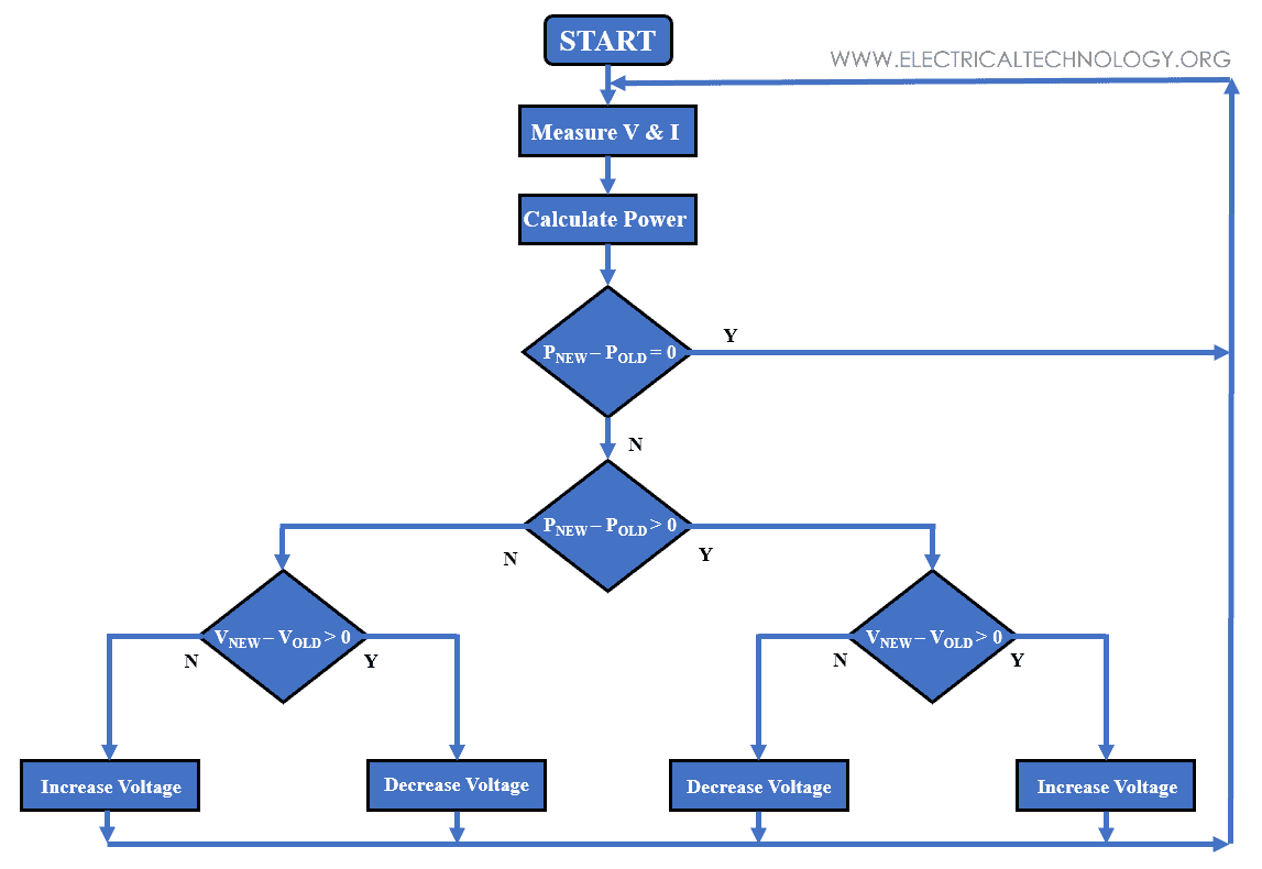
The value of PV voltage and current is measured and power is calculated. If the difference between calculated power PNEW and old calculated power POLD is zero, then the power is re-calculated else if the difference is greater than zero, it checks if there is an increase in the value of voltage by subtracting the old value of voltage VOLD from its the new value VNEW.
If the difference is greater than zero (a positive value), it means our actual operating point lies in the left region of the maximum power point and voltage needs to be increased to reach the maximum power point as shown by arrow A in figure 2. Else if the difference is less than zero (a negative value), it means that the actual operating point lies in the right of maximum power point, and decreases in the value of voltage are needed to approach the maximum power point as shown by arrow C in figure 2.
In another case, if the difference between PNEW and POLD is less than zero (negative value), it is checked whether the voltage is increasing or decreasing. If the difference between VNEW and VOLD is greater than zero, it indicates that our actual operating point lies on the right of maximum power point and voltage is needed to be decreased to reach the maximum power point as shown by arrow C in figure 2.
But on the contrary, if the difference between VNEW and VOLD is less than zero while the difference between PNEW and POLD is less than zero then our actual operating point lies on the left of maximum power point and voltage needs to be increased to reach maximum power point as shown by arrow A in figure 2.
The rate of convergence to maximum power point depends on the perturbation value. Higher the value less the time it takes to reach a maximum power point, but the higher value will result in poor accuracy as the operating point will hover back and forth at the maximum power point.
The accuracy can be improved by reducing the value of perturbation. But a decrease in the value of perturbation will result in more time for the operating point to reach maximum power point. But this method faces the drawback when the solar irradiance changes while the operating point is about to approach the maximum power point.
Let’s take a look at figure 4 to understand this, when the operating point is approaching the maximum power point it is perturbing on the logic that the present operating point is towards the left region and maximum power point A is towards the right, so the perturbation is done towards the right to reach maximum power point A.
Related Posts:
- Series, Parallel & Series-Parallel Connection of Solar Panels
- How to Wire Solar Panels in Series-Parallel Configuration?

But the change in solar irradiance changes the P-V curve of the module and the new maximum power point B is now towards the left of the actual operating point and less than the previous maximum power point value at point A.
But the algorithm perturbs the voltage towards the right based on the logic that its previous value of operating power is less than the power at point A. This results in the error and delays for our operating point to converge to its new maximum power point at point B.
Thus, this algorithm perturbs the value of voltage by adjusting the duty cycle of the power converter switching device and observers the increase or decrease in the value of power as compared to its previous value to reach the maximum power point. Hence, the name Perturb & Observe.
Related Posts:
- Parameters of a Solar Cell and Characteristics of a PV Panel
- How to Design a Solar Photovoltaic Powered DC Water Pump?
- How to Wire Batteries in Series-Parallel to a Solar Panel?
- How to Wire Batteries in Parallel to a Solar Panel and UPS?
- How to Wire Solar Panel to 12V DC Load and Battery?
- How to Wire Solar Panel to 120-230V AC Load and Inverter?
- How to Wire Batteries in Series to a Solar Panel and UPS?
- How to Wire Solar Panels & Batteries in Series-Parallel Connection?
- How to Wire Solar Panels in Series & Batteries in Parallel? 12/24/48V System
- How to Wire Solar Panels in Parallel & Batteries in Series? 24V System
- How to Wire Solar Panel & Batteries in Parallel for 12V System
- How to Wire Solar Panel & Batteries in Series for 24V System